A High efficiency Resonant Switched Capacitor Converter With Continuous Conversion Ratio

Appendix

3.1.1 Charge Flow Analysis for Different Conversion Ratios

Figure 3.21a–c shows the different capacitor configurations for the separate phases φ1 and φ2 of the proposed multi-ratio ReSC converter depending on the conversion ratio N. For each phase i, a charge multiplier vector can be defined describing the topology based on the charge flow through the capacitors.

$$\displaystyle \begin{aligned} \boldsymbol{a}^{(i)} = \left[q_{\mathrm{out}}^{(i)} \ \ q_{C_1}^{(i)} \ \ \ldots \ \ q_{C_n}^{(i)} \ \ q_{\mathrm{in}}^{(i)} \right]^{\mathrm{T}} \cdot \frac{1}{q_{\mathrm{out}}} = \left[a_{\mathrm{out}}^{(i)} \ \ a_{C_1}^{(i)} \ \ \ldots \ \ a_{C_n}^{(i)} \ \ a_{\mathrm{in}}^{(i)} \right]^{\mathrm{T}} \end{aligned} $$

(3.12)

Fig. 3.21

Charge flow analysis for the resonant multi-ratio ReSC converter: (a) conversion ratio 1/3; (b) conversion ratio 1/2; (c) conversion ratio 2/3

Full size image

With Fig. 3.21a–c, the charge multiplier vectors of the different conversion ratios can be determined:

Ratio N = 1/3

$$\displaystyle \begin{aligned} \boldsymbol{a}_{1/3}^{(1)} = \left[q_{\mathrm{x}}\ \ q_{\mathrm{x}}\ \ q_{\mathrm{x}}\ \ q_{\mathrm{x}}\right]^{\mathrm{T}} \cdot \frac{1}{3q_{\mathrm{x}}} =\left[\frac{1}{3}\ \ \frac{1}{3} \ \ \frac{1}{3} \ \ \frac{1}{3}\right]^{\mathrm{T}} \end{aligned} $$

(3.13)

$$\displaystyle \begin{aligned} \boldsymbol{a}_{1/3}^{(2)} = \left[2q_{\mathrm{x}}\ \ -q_{\mathrm{x}}\ \ -q_{\mathrm{x}}\ \ 0\right]^{\mathrm{T}} \cdot \frac{1}{3q_{\mathrm{x}}} = \left[\frac{2}{3}\ \ -\frac{1}{3} \ \ -\frac{1}{3} \ \ 0\right]^{\mathrm{T}} \end{aligned} $$

(3.14)

Ratio N = 1/2

$$\displaystyle \begin{aligned} \boldsymbol{a}_{1/2}^{(1)} = \left[2q_{\mathrm{x}}\ \ q_{\mathrm{x}}\ \ q_{\mathrm{x}}\ \ 2q_{\mathrm{x}}\right]^{\mathrm{T}} \cdot \frac{1}{4q_{\mathrm{x}}} =\left[\frac{1}{2}\ \ \frac{1}{4} \ \ \frac{1}{4} \ \ \frac{1}{2}\right]^{\mathrm{T}} \end{aligned} $$

(3.15)

$$\displaystyle \begin{aligned} \boldsymbol{a}_{1/2}^{(2)} = \left[2q_{\mathrm{x}}\ \ -q_{\mathrm{x}}\ \ -q_{\mathrm{x}}\ \ 0\right]^{\mathrm{T}} \cdot \frac{1}{4q_{\mathrm{x}}} =\left[\frac{1}{2}\ \ -\frac{1}{4} \ \ -\frac{1}{4} \ \ 0\right]^{\mathrm{T}} \end{aligned} $$

(3.16)

Ratio N = 2/3

$$\displaystyle \begin{aligned} \boldsymbol{a}_{2/3}^{(1)} = \left[2q_{\mathrm{x}}\ \ q_{\mathrm{x}}\ \ q_{\mathrm{x}}\ \ 2q_{\mathrm{x}}\right]^{\mathrm{T}} \cdot \frac{1}{3q_{\mathrm{x}}} =\left[\frac{2}{3}\ \ \frac{1}{3} \ \ \frac{1}{3} \ \ \frac{2}{3}\right]^{\mathrm{T}}\end{aligned} $$

(3.17)

$$\displaystyle \begin{aligned} \boldsymbol{a}_{2/3}^{(2)} = \left[2q_{\mathrm{x}}\ \ -q_{\mathrm{x}}\ \ -q_{\mathrm{x}}\ \ 0\right]^{\mathrm{T}} \cdot \frac{1}{3q_{\mathrm{x}}} =\left[\frac{1}{3}\ \ -\frac{1}{3} \ \ -\frac{1}{3} \ \ 0\right]^{\mathrm{T}}\end{aligned} $$

(3.18)

For the calculation of the equivalent output resistance R _out, only the corresponding charge flow of the output has to be considered

$$\displaystyle \begin{aligned} &\mathrm{Ratio\;\mathit{N}=1/3}: \quad q_{\mathrm{out,1/3}}^{(1)} = \frac{1}{3} \quad q_{\mathrm{out,1/3}}^{(1)} = \frac{2}{3} \\ &\mathrm{Ratio\;\mathit{N}=1/2}: \quad q_{\mathrm{out,1/2}}^{(1)} = \frac{1}{2} \quad q_{\mathrm{out,1/2}}^{(2)} = \frac{1}{2} \\ &\mathrm{Ratio\;\mathit{N}=1/2}: \quad q_{\mathrm{out,2/3}}^{(1)} = \frac{2}{3} \quad q_{\mathrm{out,2/3}}^{(2)} = \frac{1}{3} \end{aligned} $$

3.1.2 Calculation of the Equivalent Output Resistance for Different Conversion Ratios

3.1.2.1 Determination of the Equivalent Circuits for the Switching Phases

To set up the differential equations for the current according to the equivalent circuit for the corresponding phase as shown in Fig. 2.13b, it is necessary to determine the component values R _i , C _i for the corresponding switching phase i. This procedure is illustrated in the following for the conversion ratio 2/3. Figure 3.22a shows the resulting schematics for the phases φ1 and φ2 for the 2/3 conversion ratio. In phase φ1, both flying capacitors C _fly1 and C _fly2 are connected in parallel, which leads to a resulting capacitor value of (with )

(3.19)

In phase φ2 they are connected in series, resulting in

(3.20)

The power switches are connected in parallel in phase φ1, which leads to an effective resistance R ₁ of (assuming same on-resistance R _sw for all power switches)

(3.21)

In phase φ2, the series connection of the power switches results in

(3.22)

Accordingly, this procedure can also be applied to the other conversion ratios.

Fig. 3.22

(a) Schematic of the individual switching phases for 2/3 conversion ratio; (b) resulting equivalent circuits of the individual phases for calculation of the equivalent output resistance

Full size image

3.1.2.2 Derivation of the Current Equations for the ReSC Converter

The equivalent circuit in Fig. 2.13b leads to a homogeneous second-order differential equation with constant coefficients.

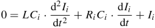
(3.23)

This can be solved easily to get the following generalized solution for the current I(t)

$$\displaystyle \begin{aligned} I\left(t\right) = \begin{cases} A_{11} \cdot \mathrm{e}^{\lambda_{\mathrm{11}} t} + A_{12} \cdot \mathrm{e}^{\lambda_{\mathrm{12}} t} & t\in \left[0,\tau_1\right] \\ A_{21} \cdot \mathrm{e}^{\lambda_{\mathrm{21}} \left(t-\tau_1\right)} + A_{22} \cdot \mathrm{e}^{\lambda_{\mathrm{22}} \left(t-\tau_1\right)} & t\in \left[\tau_1,\tau_1+\tau_2\right] \\ \end{cases} \end{aligned} $$

(3.24)

where the eigenvalues λ _ik are

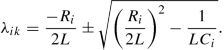
(3.25)

For the determination of the constants A _ik , four additional boundary conditions are required. The first two can be determined with the charge flow analysis. The charge \(q_{\mathrm {out}}^{(i)}\) flowing into the output in each phase i must be equal to the integral of the current over the phase τ _i

$$\displaystyle \begin{aligned} q_{\mathrm{out}}^{(i)} = a_{\mathrm{out}}^{(i)} \cdot q_{\mathrm{out}} = \int_{0}^{\tau_i} I_i(t) \mathrm{d}t \end{aligned} $$

(3.26)

Phase φ1:

$$\displaystyle \begin{aligned} a_{\mathrm{out}}^{(1)} \cdot q_{\mathrm{out}} = \dfrac{A_{11}}{\lambda_{\mathrm{11}}} \cdot (\mathrm{e}^{\lambda_{\mathrm{11}}\tau_1}-1) + \dfrac{A_{12}}{\lambda_{\mathrm{12}}} \cdot (\mathrm{e}^{\lambda_{\mathrm{12}} \tau_1}-1) \end{aligned} $$

(3.27)

Phase φ2:

$$\displaystyle \begin{aligned} a_{\mathrm{out}}^{(2)} \cdot q_{\mathrm{out}} = \dfrac{A_{21}}{\lambda_{\mathrm{21}}} \cdot (\mathrm{e}^{\lambda_{\mathrm{21}}\tau_1}-1) + \dfrac{A_{22}}{\lambda_{\mathrm{22}}} \cdot (\mathrm{e}^{\lambda_{\mathrm{22}} \tau_1}-1) \end{aligned} $$

(3.28)

The other two boundary conditions can be determined by the transition during the phases. Due to the inductor, the current at the beginning of each switching phase must be the same as at the end of the previous one. For two switching phases (i = 2), this means

$$\displaystyle \begin{aligned} I_{1,2}(t=0)=I_{2,1}(t=\tau_{2,1}){} \end{aligned} $$

(3.29)

First transition

$$\displaystyle \begin{aligned} I_1(t=0)&=I_2(t=\tau_2) \end{aligned} $$

(3.30)

$$\displaystyle \begin{aligned} A_{11} + A_{12} &= A_{21} \cdot \mathrm{e}^{\lambda_{\mathrm{21}}\tau_2} + A_{22} \cdot \mathrm{e}^{\lambda_{\mathrm{22}}\tau_2}{} \end{aligned} $$

(3.31)

Second transition

$$\displaystyle \begin{aligned} I_2(t=0)&=I_1(t=\tau_1) \end{aligned} $$

(3.32)

$$\displaystyle \begin{aligned} A_{21} + A_{22} &= A_{11} \cdot \mathrm{e}^{\lambda_{\mathrm{11}}\tau_1} + A_{12} \cdot \mathrm{e}^{\lambda_{\mathrm{12}}\tau_1}{} \end{aligned} $$

(3.33)

Equations 3.27, 3.28, 3.31, and 3.33 lead to a 4 × 4 equation system for the determination of A ₁₁ to A ₂₂. For the sake of clarity, the auxiliary variable W _ik is introduced

$$\displaystyle \begin{aligned} W_{ik} = \dfrac{e^{\lambda_{\mathrm{ik}}\tau_i}-1}{\lambda_{ik}}. \end{aligned} $$

(3.34)

With that, the equation system can be written with

$$\displaystyle \begin{aligned} \left( \begin{array}{cccc} W_{11} & W_{12} & 0 & 0 \\ 0 & 0 & W_{21} & W_{22} \\ -1 & -1 & e^{\lambda_{\mathrm{21}}\cdot\tau_2} & e^{\lambda_{\mathrm{22}}\cdot\tau_2} \\ e^{\lambda_{\mathrm{11}}\cdot\tau_1} & e^{\lambda_{\mathrm{12}}\cdot\tau_1} & -1 & -1 \\ \end{array} \right) \cdot \left( \begin{array}{c} A_{11}\\ A_{12}\\ A_{21}\\ A_{22}\\ \end{array} \right) = \left( \begin{array}{c} a_{\mathrm{out}}^{(1)} \cdot q_{\mathrm{out}} \\ a_{\mathrm{out}}^{(2)} \cdot q_{\mathrm{out}} \\ 0 \\ 0 \\ \end{array} \right). \end{aligned} $$

(3.35)

With Eq. 3.35, the coefficients A ₁₁, A ₁₂, A ₂₁, and A ₂₂ can be calculated and inserted in Eq. 3.24. The current I _i can then be used in Eq. 2.14 for calculating the equivalent output resistance of a ReSC converter. Since the symbolic solution for R _out in the general case leads to a very complex equations, MATLAB^® is used for solving the system of equations and the final R _out calculation.

3.1.3 Implementation of an Additional Conversion Ratio 4/7 by Three-Phase Operation

Figure 3.23 shows the different capacitor configurations for the three separate phases φ ₁, φ ₂, and φ ₃ of the proposed 4/7 ratio power stage (see Fig. 3.4) along with the parameters from the charge flow analysis (see Sect. 2.3.1).

Fig. 3.23

Charge flow analysis for the 4/7 conversion of the resonant SC converter

Full size image

With Fig. 3.23, the charge multiplier vectors for the different phases can be determined

$$\displaystyle \begin{aligned} \boldsymbol{a}_{4/7}^{(1)} = \left[4q_{\mathrm{x}}\ \ 3q_{\mathrm{x}}\ \ q_{\mathrm{x}}\ \ q_{\mathrm{x}} \ \ 4q_{\mathrm{x}}\right]^{\mathrm{T}} \cdot \frac{1}{7q_{\mathrm{x}}} =\left[\frac{4}{7}\ \ \frac{3}{7} \ \ \frac{1}{7} \ \ \frac{1}{7} \ \ \frac{4}{7}\right]^{\mathrm{T}} \end{aligned} $$

(3.36)

$$\displaystyle \begin{aligned} \boldsymbol{a}_{4/7}^{(2)} = \left[2q_{\mathrm{x}}\ \ -2q_{\mathrm{x}}\ \ -2q_{\mathrm{x}}\ \ 0 \ \ 0 \right]^{\mathrm{T}} \cdot \frac{1}{7q_{\mathrm{x}}} =\left[\frac{2}{7}\ \ -\frac{2}{7} \ \ -\frac{2}{7} \ \ 0 \ \ 0\right]^{\mathrm{T}} \end{aligned} $$

(3.37)

$$\displaystyle \begin{aligned} \boldsymbol{a}_{4/7}^{(3)} = \left[q_{\mathrm{x}}\ \ -q_{\mathrm{x}}\ \ q_{\mathrm{x}}\ \ -q_{\mathrm{x}} \ \ 0 \right]^{\mathrm{T}} \cdot \frac{1}{7q_{\mathrm{x}}} =\left[\frac{1}{7}\ \ -\frac{1}{7} \ \ \frac{1}{7} \ \ -\frac{1}{7} \ \ 0\right]^{\mathrm{T}} \end{aligned} $$

(3.38)

The ratio of the total input and output charge elements leads to the desired conversion ratio 4/7

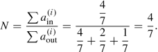
(3.39)

According to the charge flow analysis, the flying capacitor C _fly3 delivers the smallest amount of charge. Therefore, the existing power stage (see Fig. 3.1) with 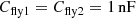is extended by a small 250pF capacitor for C _fly3 as shown in Fig. 3.4b. Due to different voltage polarities across the power switches during operation, the power switches S2, S7, and S9 have to be implemented by a back-to-back transistor configuration.

Depending on the capacitor configuration in each phase, different resonance frequencies occur, which also lead to different duty cycles (see Sect. 3.1). This can be seen in Fig. 3.24, where the simulated transient waveforms of the inductor current I _L and the clock signals φ1, φ2, and φ3 are shown. The inductor current I _L in the individual phases matches the calculated output charge vectors (\(a_{\mathrm {out,4/7}}^{(1)}=4/7\), \(a_{\mathrm {out,4/7}}^{(2)}=2/7\), \(a_{\mathrm {out,4/7}}^{(3)}=1/7\)). The amount of charge is halved after each phase. The benefit of the 4/7 conversion ratio can be seen in Fig. 3.4a, where the simulated converter efficiency is plotted over the input voltage V _in. The 4/7 ratio leads to an efficiency improvement of up to 7%.

Fig. 3.24

Simulated transient waveforms of the 4/7 conversion ratio for , , : (a) inductor current I _L; (b) clock signals φ1, φ2, and φ3

Full size image

southrinte1987.blogspot.com

Source: https://link.springer.com/chapter/10.1007/978-3-030-63944-0_3

Share this post